Dont Drift Out of ControlPart 2

There is a perceived market need, dictated by the FDA, to maintain the accuracy of sensors that are defined as current Good Manufacturing Practices (cGMP) values in a validated pharmaceutical process. Today, this is achieved by maintaining a costly routine calibration protocol.

In Part 1 of this article (“Don’t Drift Out of Control,” October 2008), I introduced an aggressive technique to shift from routine preventive maintenance methodology (i.e., to calibrate an instrument every six months regardless of past experience) to a predictive maintenance methodology using pairs of instruments and performing a statistical analysis of their behavior. When the statistical analysis recognizes that at least one of the instruments is beginning to drift away from its paired instrument, an alarm message can be sent to the metrology department to schedule a calibration of both instruments.

The upside of this technique is that it will detect drifting instruments in real time, thus eliminating the need for non-value-added routine calibrations that can be 50% of the metrology department’s budget, and will provide immediate notification of a developing calibration problem before the instrument and the related product quality parameter goes out of specification.

The downside is the capital expense to add a second instrument to any validated instrument where you elect to adapt this technique. At first blush this will appear to be a belt-and-suspenders solution, but it is necessary in order to detect common cause failures that will have to be addressed if you elect to depend on a predictive rather than a preventive maintenance strategy. However, the economic justification is certainly there for instruments where product quality is a major issue or where the cost of a routine calibration is very expensive, such as in a hazardous area.

This leads to a more practical question: What can a statistical analysis provide without the cost of the additional instruments? The answer may surprise you. There is hidden data in an instrument’s signal that can provide an indication that an instrument’s behavior has changed. This phenomenon can be used to predict the need for calibration and therefore capture the second benefit of detecting a drifting instrument before it affects quality. Since it’s a single instrument solution, it is unlikely to totally eliminate periodic calibrations, but it can provide quantifiable data to justify a longer interval between calibrations. The hidden data is the variance in the instrument’s signal.

Calibration Basics
Let us begin by establishing a base level of understanding of instrumentation calibration.

Precise, dependable process values are vital to an optimum control scheme and, in some cases, they are mandated by compliance regulation. Precision starts with the selection and installation of the analog sensor while the integrity of the reported process value is maintained by routine calibration throughout the life of the instrument.

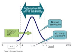
When you specify a general purpose instrument, it has a stated accuracy—for example, +/- 1% of actual reading. In the fine print, that means that the vendor states that the reading of the instrument will be within 1% of reality 95% of the time (certainty). Figure 1 illustrates this concept.

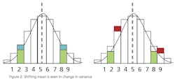
Variance, or standard deviation, which is the square root of variance, is an indication of the shape of a bell curve of a normal distribution of sample data. The more the data is concentrated around the medium average, the smaller the variance and the skinnier the bell curve. Conversely, the wider the distribution of the data, the larger the variance and the fatter the bell curve.InsightsThe first key insight to recognize here is that for a given instrument in good working order, it will have a characteristic variance and bell curve shape. A highly accurate instrument will have a tall skinny bell curve where a less accurate instrument will have a wider bell curve.The next key insight is that an instrument will exhibit this characteristic distribution whenever the instrument is sensing a steady state parameter and will exhibit a repeatable different characteristic distribution when the sensed parameter is not holding constant.Suppose you have a flow meter that is reading exactly 6 liters per hour and then the flow rate experiences a step change from 6 to 7 liters per hour. Given sufficient time to collect a sample, the standard deviation of the instrument around the mean value “6” will be identical to the standard deviation around the mean value “7” (assuming that “6” and “7” are within the linear operating range of the instrument). Interestingly, as it is transitioning from “6” to “7”, it is flushing out old values from its FIFO (first in, first out) history file and replacing them with values centered around the new reality, “7”. Figures 2 and 3 demonstrate this interesting statistical phenomenon.

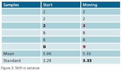
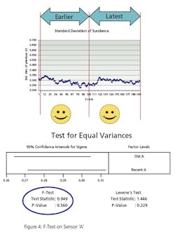
When a sample is shifting from one mean to another, the variance increases during the transition period. In this example, two pieces of data, a “2” and an “8”, shifted a mere one unit to the right to become a “3” and a “9”. The result is that the mean shifted to the right—from 5.0 to 5.33—and the standard deviation also shifted up from 3.29 to 3.33.During this transition period, the standard deviation increases in a characteristic manner and then eventually settles back to the steady state standard deviation.We use this shift to detect drift. The actual mean value of the sample is of little consequence to the task of detecting instrument drift. The operator and the computer control programs see the most recent sensed value and conduct operations on that value, not the sample mean.The new insight here is that an unusual change in the variance’s behavior is the criteria to suspect an instrument has experienced a change in performance characteristics (i.e., may be starting to drift) and deserves to be calibrated.Variance should maintain statistical consistency over time. An instrument’s integrity becomes suspect when there is a significant change in its variance (up or down). If it has gained variance relative to its past, it is becoming erratic or unstable. If it has lost variance, it is becoming insensitive or may have fouled. Proof of ConceptThe statistical test to determine whether a sensor is experiencing a failure is the F-test. The hypothesis is that the failing sensor can be detected by a change in the variance of the sample. The technique is to accumulate a large historical file of instrument readings—say 1,000—then subgroup the sample into groups of 25 and calculate each subgroup’s variances. Then compare the variances of the subgroups of the oldest 500 samples with the newest 500 samples. If the sensor is experiencing change it will fail the F-test.Figure 4 is an example using the data that was presented in Part I of this article. Instrument A has a history file of 1,000 samples with instrument noise simulated by a random number generator. The first test compares the variance of instrument A’s oldest 500 values to its most recent 500 reading. The F-Test p-Value of .560 (>.05) indicates that the variances are “equal,” which is correct. Therefore, this instrument is performing as usual.

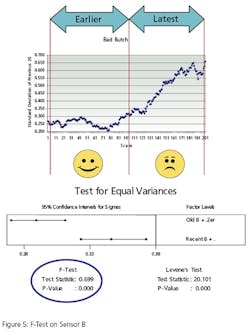
The second test, Figure 5, conducts the same test on a different instrument. It compares the variance of instrument B’s oldest 500 values to its most recent 500 reading. Instrument B has bias superimposed on its last 500 values to simulate error. The F-Test p-Value of .00 (>.05) indicates that the variances are “different”.

Since instrument “B” does seem to be changing, we can issue an advisory that declares “B” is suspect and we can predict the need for a calibration.Therefore, the use of the F-test can be used to detect change in the instrument’s characteristic behavior that is a harbinger of an instrument beginning to drift. This early warning can be used to trigger an early calibration and eliminate off-spec production.Economic JustificationFurthermore, although the F-test is only an advisory for single instrument situations and cannot totally eliminate scheduled preventive maintenance as is suggested with a two-instrument/control chart technique that was described in Part 1 of this article, it can be used to extend the calibration interval. Given enough instrument history—say 3-4 years—of a high correlation between change in variance and instrument drift and, conversely, no correlation between no change in variance data and “calibration not needed” reports from self-imposed preventive maintenance calibrations, one could extend the preventive maintenance scheduled calibration periods from, say, six months to one year. This would cut the preventive maintenance schedule calibration budget in half without adding the second set of instruments. Today, data integrity is maintained by rigid adherence to a preventive maintenance program and a set of secondary protocols that address potential product quality issues that may arise when a validated instrument is detected be out of calibration. In the future, metrology department cost and responsiveness can be improved by scheduling calibrations as a function of the statistical analysis of past experience, a predictive maintenance philosophy. This will increase the time between calibrations where appropriate and reduce the exposure to off spec product by early detection of potential loss of instrument integrity.In conclusion, the FDA has been encouraging the use of statistics and other technologies as part of the PAT initiative. This article has demonstrated that we can dramatically improve the data integrity of the critical (cGMP) instrument signals through statistical analysis and reduce calibration cost by setting the calibration interval based on past experience. Significant improvements in data integrity will reduce the life cycle cost of the calibration functions and minimize the downside risk of poor quality or lost production caused by faulty instrumentation—the very spirit of PAT.General ReferencesCable, Mike. Calibration: A Technician’s Guide. ISA 2005.Chowdhury, Subir. Design for Six Sigma. Dearborn Trade Publishing 2002. Dieck, Ronald H. Measurement Uncertainty: Methods and Applications, Third Edition. ISA 2002. Friedmann, Paul G. Economics of Control Improvement. ISA 1995.Hashemian, H.M. Sensor Performance and Reliability. ISA 2005.Sincich, T., Levine, D., Stephan, D. Practical Statistics by Example Using Microsoft Excel and Minitab, Second Edition. Prentice-Hall 2002.Van Beurden, Iwan. “System Availability Evaluation” version V1, revision R2. A white paper by Exida, May 5, 2005.About the AuthorDan Collins is a certified Six Sigma Black Belt with over thirty-five years of experience in industrial process and control. He is currently an adjunct professor of engineering at Montgomery County Community College in Blue Bell, Pennsylvania. Mr. Collins holds a B.B.A. in marketing from the University of Notre Dame, a B.A. in physics from Temple University, an M.E. in industrial engineering from Penn State University and an M.B.A. from Rutgers University.