Estimating Risk-Based Cost and Contingency

Sept. 5, 2012
How to Apply Monte Carlo Simulation to Engineering Capital Projects

Estimating capital project budgets can be a tricky business. There are many factors to include as inputs to the budget: vendor quotes, capital labor, permits, third- party inspections, expenditure data from previous projects, material escalation… the list goes on and on. Unfortunately, each input can itself be an estimate, and each input can present cost uncertainty risks. Because it is impossible to calculate a precise, infallible budget (owing to the nature of project risk and cost uncertainty), numerical analysis is a good option for arriving at a solution. In the case of predicting capital budgets, the Monte Carlo Simulation (MCS) is the numerical method of choice.

What is a MCS? In terms of project cost risk, the MCS is a tool for calculating the statistical likelihood of exceeding a base budget by a given value. The goal is to assign a statistically-derived dollar value to the various risks associated with the project. The MCS calculates budget values and likelihoods based on two key inputs for each budget line item: 1) the forecasted cost distribution for the expenditure, and 2) the chance of incurring the expenditure.For example, Item A should cost between $70,000 and $85,000, and there is a 100% of incurring the cost; Item B should cost between $10,000 and $15,000, but there is only an 80% chance of incurring the cost. (Table 1).

Table 1: Example Monte Carlo InputsThe MCS generates random numbers and applies them to the cost and likelihood-of-occurrence for each line item. The sum of all line items is a resulting budget scenario - also called an iteration. The first iteration may yield a budget of $93,561 because Item B occurs. The second iteration may yield a budget of $74,829 because Item B doesn’t occur.

Table 2: Example Monte CarloUsing this random “roll of the dice” calculation method, the MCS generates thousands of budget iterations. A simple results chart then tabulates the iterations and calculates the budget contingency required to have X% certainty of staying within budget. MCS overall results typically read like this: for a $90,000 baseline budget, a contingency of $2,950 should be allocated to assure that the project doesn’t go overbudget – assuming management accepts an 80% likelihood of staying within budget. For a 90% likelihood of staying within budget, the MCS may calculate that $5,820 contingency is required.At this point, many project managers and engineers will say, “OK, fine, I’ll try using a MCS to estimate my budget – where can I download one, and how much does it cost?” There certainly are commercially- available MCS software packages, and some are very affordable (less than $100 for a single license). The problem lies in using a black-box method to estimate a budget. Regardless of how poorly or how well a MCS package performs, it is likely that the end user doesn’t fully understand its internal workings. What probability distributions are used? Is the random number generator truly random? How many iterations are performed? For that matter, how many iterations are required?...For those willing to remove the MCS from within its black box, the rewards are great. The only requirements for creating a MCS from scratch are: 1) a spreadsheet program, 2) familiarity with basic spreadsheet functions, and 3) following along with the example below. The end product will be a MCS spreadsheet that is user-friendly, documented, fully understood, and similar in function to commercially- available options. Still reading?... let’s begin!Building Your Own MCS ToolThe most important aspect of understanding MCS mechanics is knowing how to generate meaningful cost probability distributions. There are many probability distributions that could be used to describe forecasted cost: normal distribution (standard bell curve), uniform distribution (see Table 2), log-normal distribution, beta distribution, etc. The problem lies in translating straightforward cost data into statistical distribution lingo. It takes a skilled statistician to, for example, analyze limited data and generate the α and β parameters of a beta distribution. Moreover – how does “α=2, β=5” translate to a $10,000,000 line item? The beta parameters have no clear meaning on the surface.Fortunately, there exists a straightforward and easy-to-generate distribution that is well suited to MCSs: the triangular distribution (TriD). A TriD has three simple parameters: low limit a, high limit b, and likely value c. The TriD’s Probability Distribution Function (PDF – a function that describes the likelihood of a random variable having any given value) shows the characteristic triangular shape, with the “likely value” having the highest chance of occurring. The chance of occurring drops to 0% at the high and low values. (Figure 1).
The TriD is a good choice for MCSs for multiple reasons. Firstly, the parameters (a, b, c) used to define the distribution are easily superimposed onto a budget line item: Lowest possible cost, highest possible cost, and most likely cost, respectively. This aids in easy comprehension of the cost inputs. Additionally, the triangular shape of the distribution is versatile enough to approximate forecasted cost for a variety of possible line items. For example, “time & material” line items can place the Likely Cost centrally between the Low and High Costs (roughly approximating a bell curve) – this accounts for the risk of either less or more T&M cost. For lump-sum and not-to-exceed budget items, the Likely Cost can be set closer to (or equal to) the High Cost, indicating low likelihood of exceeding the line item cost. If using expired vendor quotations to forecast future projects, the Likely Cost can be set equal to the Low Cost, indicating likelihood of future cost being higher than current benchmark data.Important Note: For each line item, the MCS user must carefully consider the Low, High, and Likely values. Obtaining early consensus on MCS inputs with vested internal parties can prevent questions and challenges in later project stages.Returning to the previous MCS input example (Table 1), Item A was assigned a low limit of $70,000 and a high limit of $85,000. To generate a TriD for Item A, the only missing input is assignment of the likely value. Assuming that a vendor has quoted Item A at $75,000, our TriD specification is complete (a=$70,000, b=$85,000, c=$75,000). The only remaining hurtle is to transform the three TriD parameters into a randomly-generated cost data sample that takes on the triangular distribution when tabulated.Using a spreadsheet’s random number generator, infinite random decimal numbers between 0 and 1can be created. Kotz and van Dorp provide the equations necessary to transform this random variate into a triangular distribution with Low Value = a, High Value = b, and Likely Value = c. The TriD transformed line item cost “CostTriD” for a random cost variable x in any iteration is given by Equations 1 and 2 (for 0 ≤ x ≤ 1):

Because the likelihood of occurrence may not be 100% for all line items, an additional check is performed to determine if the line item’s cost is included in the iteration total cost. The assigned iteration cost “CostI” of each line item, based on random occurrence variable y is given by Equations 3 and 4 (for 0 ≤ y ≤ 1):

When translated to spreadsheet language, Equations 1-4 can be condensed to this formula:
By referencing previously entered TriD inputs (a, b, c, and likelihood), along with two long columns of random numbers (x and y for each iteration), Formula 1 will generate the TriD data points for each line item. To transform this data set into a meaningful visual representation, the individual points must be sorted into a Cost Frequency Distribution – a graph showing how frequently the CostI results fall into various cost brackets. To accomplish this, create a column of 20 numbers: from the line item’s Low Value to High Value, with intervals of (High-Low)/20. This column will be the values of the x axis for the cost frequency distribution. To sort each randomly generated CostI into a cost frequency distribution bracket, a vlookup is performed:
Assuming 1,000 iterations were calculated, Formula 2 will be used to sort each of the 1,000 Cost I values into a cost bracket. This creates a column of 1,000 numbers, each being a value from the list of 20 brackets. Now, a CountIf formula can be used to tally the Formula 2 results for each of the 20 brackets:
By graphing the Formula 3 results against the list of 20 bracket values, a visual representation of the TriDis created:

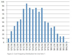
In figure 2, each bar represents the number of data points randomly generated between the indicated x axis value and the next higher x axis value. For example, 51 data points fall between Cost I of $79,000 and $79,750. Only 2 data points fall between $84,250 and $85,000. It should be noted that Figure 2 does not take on a perfectly triangular shape – this is to be expected. Because the dataset is based on a random number generator, there is an extremely small likelihood of the triangle being perfectly formed. For Figure 2, 1,000 data points were used. For a sample size of only 100 data points, the triangle shape would be must less pronounced. For a sample size of 50,000 data points, the triangle would appear much more precisely formed.Now that the TriD is generated (and visually verified) for line item 1, the same methodology is used to create the TriDs for each line item. Using the F9 key to refresh the calculations will update the random numbers, and will show how variable the triangular shape can be. Note, however, that the peak will always be at or near the Likely Value assigned to each line item, and the trend will decrease to 0 at the Low and High limits.Let’s speculate that our MCS is being created for a vessel procurement project. A new agitated process vessel must be purchased and connected to an existing piping system, but there is a 20% chance that the agitator can be sourced internally from   decommissioned vessel at another site. The MCS input is defined as:

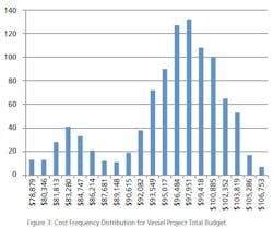
Table 3: VesselUsing the methods described above, a 1,000 iteration MCS results table is generated, and the Cost Frequency Distribution graph for each line item indicates that the calculations are behaving as intended. To generate the MCS total budget, the CostI of each line item is simply summed for each iteration into a column of 1,000 budget total data points. The 20 bracket values for the budget total data set can be determined by using the MIN() and MAX() functions and referencing the range of budget totals. By applying the vlookup and countif methods to the budget total data column (use [MAX()-MIN()]/20 to determine the bracket intervals), a cost frequency distribution for the overall budget can be generated:
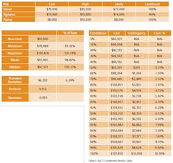
Because not all line items had a 100% chance of occurring, the cost frequency distribution shows a dip that might not have been anticipated without the use of a MCS. Though illustrative, Figure 3 does not provide the critical result that will determine the final budget and contingency. The final budget result comes from using a few simple statistical analysis functions.To form the baseline budget (Base Cost) against which analysis is performed, the Likely values are summed. The following spreadsheet functions (referencing the column of total budget results) will yield informative statistical indicators: MIN(), MAX(), AVERAGE(), MEDIAN(), STDED.P(), KURT(), SKEW(). See Table 4 below for examples of these calculations (reference the spreadsheet’s help file for function descriptions). Dollar-value statistical indicators are calculated as a percentage of the Base Cost, showing the variability present in the iterations.

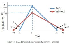
The most relevant MCS result is calculated in the cost confidence table (See Table 4). The cost confidence table uses a simple formula to calculate the total budget required to guarantee an X% chance of staying within budget: PERCENTILEINC([dataset],[percentile]). This function references the range of 1,000 budget total data points as the [dataset], along with a desired confidence [percentile]. The formula’s result is the budget value that falls at the desired percentile. For example, at the 90 th percentile (90% of the budgets calculated fall below this budget), the total budget happens to be $102,677. Comparing this to the Base Cost of $97,000, a contingency of $5,677 should be allocated. It is also helpful to calculate each percentile’s contingency as a percentage of the Base Cost. The only subjective decision is to select the cost confidence percentile that is acceptable to management.Important Note: This MCS example was performed with 1,000 iterations for illustrative purposes. To increase statistical robustness of the MCS result, the MSC spreadsheet creator should consider using a very large number of iterations: targeting a minimum of 20,000. 50,000 iterations or more are desirable (but will result in a large filesize of the spreadsheet – not really a concern in this age of inexpensive storage).For the spreadsheet power-user, there is a method of transforming the standard TriD into a Modified TriD (TriMod) – similar to the TriGen function in the Excel @Risk add-on. The TriMod allows the user to specify a small chance of under- of over-running the budget line item. This is useful in cases where there is low confidence in the selected High and Low cost inputs. The TriMod calculations determine the new High and Low values that would be required to generate the desired percentages of area outside the original High and Low values. See Figure 4: The area of right-triangle θ represents the percentage of the TriMod triangle that falls outside of Low value a, and inside of new Low value m. The area of right- triangle Φ represents the percentage of the TriMod triangle that falls outside of High value b, and inside of new High value n.

By geometrically analyzing the areas of θ and Φ, the TriMod High and Low values can be calculated:
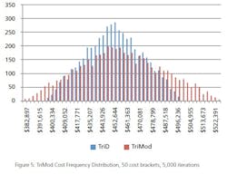
By substituting the right-hand-side of Equation 10 into all instances of n in Equation 9, m is expressed as a function of itself. By using a brute-force iterative guessing method, the value of m can be calculated [ie, a table of 2 columns: m and f(m), where each new m is guessed based on approaching the last calculated f(m)], and entered into Equation 10 to obtain n. By solving for m and n, the original (a,b,c) of the TriD have been transformed into the (m,n,c) of the TriMod. Figure 5 below shows an example a TriMod superimposed on its TriD basis: a=$400,000; b=$500,000; c=$450,000; θ=3%; Φ=7%.
Figure 5 illustrates the TriMod’s 3% chance of under-running the Low input of $400,000, and 7% chance of over-running the High input of $500,000.Whether a TriD or a TriMod is used as the basis for a MCS, the user can be confident in the resulting contingency amount. Project execution professions will appreciate the robustness of the method, and management will appreciate the confidence with which a final budget is presented. Most importantly, all methods and data will stay internal, and will be based on proprietary internally-generated tools.

References:
Kots, Samuel, and Johan Rene van Dorp. Beyond Beta – Other Continuous Families of Distributions with Bounded Support and Applications. Singapore: World Scientific Publishing Co, 2004. Print.

About the Author:
Keith Melchiors is currently a process engineer at Biogen Idec in Research Triangle Park, North Carolina. During the writing of this article, he was senior process engineer with Integrated Process Technologies in Cary, N.C. Keith earned his B.S. ChE from Purdue University in 2002, and has 10 years experience in biopharmaceutical process design and capital project execution.

Related article:
Quantifying Breakeven Point with Contingencies
About the Author

Keith Melchiors | Keith Melchiors